重温经典
2005 年,Hans Rosling(汉斯·罗琳) 和儿子 Ola Rosling、儿媳 Anna Rosling Rönnlund 一起创立了非营利性机构 Gapminder (https://www.gapminder.org/),愿景是建立基于事实的世界观,理解不断变化的世界,网站名字 gap minder 原意是提醒乘客小心站台和列车之间的间隙,笔者觉得意在提醒大家关注差异、理解变化。2006 年汉斯在 TED 做了一场演讲 — The best stats you’ve ever seen,期间展示了一系列生动形象的动画,用数据呈现的事实帮助大家解读世界的变化,可谓是动态图形领域的惊世之作。有两个令我印象深刻的点:
找最具代表性的指标,抓最能引起观众共鸣的点,用数据生动活泼地阐述一些先入为主的偏见,如发达国家收入高、寿命长,发展中国家收入中等、寿命较长,不发达国家收入低、寿命短、婴儿死亡率高、家庭成员多等。从主观印象出发,收集尽可能准确的数据,包括开放组织的数据和实验收集的数据。从一些看似简单实则富含统计和因果推理的实验中,发现一系列反偏见的结论。
在问卷里,成对的两个国家的婴儿死亡率之间至少有两倍的差距,以确保数据之间的差距远大于数据本身的误差。将问卷对象从学生扩展到教授,再拿大猩猩做对照,整个实验既有生动性又有戏剧性,强烈的反差给观众留下深刻的印象,真是一个精彩的数据故事。
图 1: 汉斯用气泡图描述儿童存活率(健康)与人均 GDP (金钱) 的关系
数据可视化在数据科学中扮演数据探索、展示和交流的关键角色,动态图形包含的信息更加丰富,在合适的数据集和应用场景上,说不定还能像汉斯那样收到奇效。《动画制作与 Plotly Python》 曾用 plotly 尝试复现汉斯展示的动态气泡图,描述数据间的关系变化。《R 语言制作地区分布图及其动画》曾分别使用 gganimate 包和 echart4r 包来制作关于地区分布图的 GIF 动画和 Web 动画,用动画描述数据的空间分布变化。
点击显示或隐藏代码
图 2: 用 echarts4r 包和 gapminder 包复现汉斯·罗琳的动态气泡图
上图2和下图3分别是采用 echarts4r 和 gganimate 包(Pedersen and Robinson 2020)绘制的,数据来自 gapminder 包(Bryan 2017),就动画制作来说,到这就差不多了。而笔者一贯的风格是要搞清楚数据来龙去脉,理解故事背后的故事,10 年后,一次偶然的机会再看汉斯·罗琳的演讲,这正是个深入了解如何动态地可视化数据关系和数据分布的机会。
点击显示或隐藏代码
library(gganimate)
ggplot(gapminder, aes(gdpPercap, lifeExp, size = pop, colour = country)) +
  geom_point(alpha = 0.7, show.legend = FALSE) +
  scale_color_manual(values = country_colors) +
  scale_size(range = c(2, 12)) +
  scale_x_log10(labels = scales::label_log()) +
  facet_wrap(~continent) +
  labs(title = "{frame_time} 年", x = "人均 GDP", y = "预期寿命") +
  theme_minimal(base_family = "Noto Sans") +
  theme(title = element_text(family = "Noto Serif CJK SC")) +
  transition_time(year) +
  ease_aes("linear")
图 3: 预期寿命和人均 GDP 的关系:从健康和经济的关系看发展中国家和发达国家
本文要抛开一些工具内置的玩具数据集,无论是 R 包 gapminder 还是 Python 模块 plotly,从找数据开始,认真理解和复现汉斯的动画,只有这样才能掌握应用动画的精髓。气泡图作为散点图的升级版,动态气泡图又是气泡图的豪华升级版,描述数量关系及其变化的核心作用没有变。除了复现汉斯的动态气泡图,还要根据数据情况,选择一些其它可视化的方式,比如用密度曲线图描述数据的分布,用岭线图描述分布的变化,还可以用动态的密度曲线图复现汉斯的另一个关于世界收入分布的动画。因此,本文接下来分五个部分介绍:
软件准备:简要介绍本文涉及的数据获取、分析、处理和可视化所需要的一系列 R 包。
数据准备:详细介绍获取和处理数据的过程。
数据探索:以 2001 年的数据为例,探索和复现汉斯·罗琳的气泡图和密度分布图。
数据展示:在探索的基础上,借助多种图形展示数据间的关系和变化趋势。
本文小结:从数据分析和技术实现方面谈一点本文写作过程中获取的经验教训。
软件准备
先安装 Noto 字体系列的两个字体包,即简体中文版的宋体字和无衬线的英文字体。在 Mac 系统下安装起来非常简单,一行命令如下:
brew install font-noto-serif-cjk-sc font-noto-sans接着,调用 sysfonts 包(Qiu 2022)加载上面安装的 Noto 系列字体,包括中文宋体和英文无衬线字体。然后,showtext 包(Qiu 2015)就可以调用系统中、英文字体处理图形中的中、英文字符。
## 简体中文宋体字
sysfonts::font_add(
  family = "Noto Serif CJK SC",
  regular = "NotoSerifCJKsc-Regular.otf",
  bold = "NotoSerifCJKsc-Bold.otf"
)
## 无衬线英文字体
sysfonts::font_add(
  family = "Noto Sans",
  regular = "NotoSans-Regular.ttf",
  bold = "NotoSans-Bold.ttf",
  italic = "NotoSans-Italic.ttf",
  bolditalic = "NotoSans-BoldItalic.ttf"
)
因 showtext 包尚不支持 gganimate 包制作中文 GIF 动画,需要使用 ragg 包,它提供新的图形设备,可以直接调用系统安装的字体,在本文源文档中,凡是使用 gganimate 的地方,添加代码块选项 dev = 'ragg_png' 即可。总体来说,本文主要使用的 R 包有:
gapminder 包(Bryan 2017): Jennifer Bryan 摘录自 gapminder 网站的数据,数据不更新,仅做部分演示。
wbstats 包(Piburn 2020):从世界银行数据库获取 1960 - 2021 年各个国家的预期寿命、人均 GDP和人口总数数据。
showtext 包(Qiu 2015):加载 Noto 系列中英文字体,供 ggplot2 包绘制静态图形。
ragg 包(Pedersen and Shemanarev 2022):加载系统 Noto 系列中英文字体,供 gganimate 包绘制 GIF 动态图形。
ggplot2 包(Wickham 2022):复现 2001 年汉斯·罗琳制作的气泡图1等。
ggrepel 包(Slowikowski 2021):缓解 ggplot2 包绘制的图形中文本重叠问题,用于复现图1。
ggridges 包(Wilke 2021):绘制岭线图,比如 1960-2020 年世界人均 GDP 分布变化图。
gganimate 包(Pedersen and Robinson 2020):人均 GDP 与寿命关系的气泡图动画(GIF 版)。
echart4r 包(Coene 2022):人均 GDP 与寿命关系的气泡图动画(Web 版)。
数据准备
R 包 gapminder 内置的数据集摘录自网站 https://www.gapminder.org/,包含 1952-2007 年142 个国家的预期寿命、总人口、人均 GDP 数据,摘录间隔是 5 年,用于 gganimate 包的帮助文档,介绍动画制作过程,乃至教学培训,都是非常合适的。
gapminder 包开发者 Jennifer Bryan 明确告诉大家她不会更新数据集,更不适合作为社会经济数据来做分析。笔者特别不喜欢分析第三手的数据,经过一番查找,发现世界银行提供相关数据,且 wbstats 包提供函数 wb_indicators() 可以查询开放的数据指标,目前有 19246 个,也提供函数 wb_data() 获取各个年份数据。下面获取各个国家自 1960 年至今的一些宏观经济指标,比如新闻里常见的人口总数、人均 GDP、预期寿命、Gini 指数、消费价格指数、通货膨胀率等。
# 从世界银行数据库获取宏观经济数据
wb_world_indicator <- wbstats::wb_data(
  indicator = c(
    "SL.UEM.TOTL",  # 失业人数 Number of people unemployed
    "SL.UEM.TOTL.ZS", # 失业率 Unemployed (%) (modeled ILO estimate)
    "SL.UEM.TOTL.NE.ZS", # 失业率 Unemployed (%) national estimate

    "NY.GDP.PCAP.KD.ZG", # 人均 GDP 增速
    "NY.GDP.MKTP.CD",# GDP 总量
    "NY.GDP.MKTP.KD.ZG", # GDP 增速

    "FP.CPI.TOTL", # 消费价格指数(以 2010 年为对比基数 100)
    "FP.CPI.TOTL.ZG", # 通货膨胀率
    "SI.POV.GINI", # Gini 指数

    "SP.DYN.LE00.IN", # 预期寿命
    "NY.GDP.PCAP.CD", # 人均 GDP
    "SP.POP.TOTL" # 人口总数
  ),
  country = "countries_only",
  return_wide = FALSE,
  start_date = 1960, end_date = 2021
)
# 保存数据到本地,方便后续使用
saveRDS(wb_world_indicator, file = "wb_world_indicator.rds")
先看下获取的数据情况:
str(wb_world_indicator)
# tibble [147,994 × 11] (S3: tbl_df/tbl/data.frame)
#  $ indicator_id: chr [1:147994] "SL.UEM.TOTL.ZS" "SL.UEM.TOTL.ZS" "SL.UEM.TOTL.ZS" "SL.UEM.TOTL.ZS" ...
#  $ indicator   : chr [1:147994] "Unemployment, total (% of total labor force) (modeled ILO estimate)" "Unemployment, total (% of total labor force) (modeled ILO estimate)" "Unemployment, total (% of total labor force) (modeled ILO estimate)" "Unemployment, total (% of total labor force) (modeled ILO estimate)" ...
#  $ iso2c       : chr [1:147994] "AF" "AF" "AF" "AF" ...
#  $ iso3c       : chr [1:147994] "AFG" "AFG" "AFG" "AFG" ...
#  $ country     : chr [1:147994] "Afghanistan" "Afghanistan" "Afghanistan" "Afghanistan" ...
#  $ date        : num [1:147994] 2021 2020 2019 2018 2017 ...
#  $ value       : num [1:147994] 13.3 11.7 11.2 11.2 11.2 ...
#  $ unit        : chr [1:147994] NA NA NA NA ...
#  $ obs_status  : chr [1:147994] NA NA NA NA ...
#  $ footnote    : chr [1:147994] NA NA NA NA ...
#  $ last_updated: Date[1:147994], format: "2022-05-25" "2022-05-25" ...
head(wb_world_indicator)
# # A tibble: 6 × 11
#   indicator_id   indicator      iso2c iso3c country  date value unit  obs_status
#   <chr>          <chr>          <chr> <chr> <chr>   <dbl> <dbl> <chr> <chr>
# 1 SL.UEM.TOTL.ZS Unemployment,… AF    AFG   Afghan…  2021  13.3 <NA>  <NA>
# 2 SL.UEM.TOTL.ZS Unemployment,… AF    AFG   Afghan…  2020  11.7 <NA>  <NA>
# 3 SL.UEM.TOTL.ZS Unemployment,… AF    AFG   Afghan…  2019  11.2 <NA>  <NA>
# 4 SL.UEM.TOTL.ZS Unemployment,… AF    AFG   Afghan…  2018  11.2 <NA>  <NA>
# 5 SL.UEM.TOTL.ZS Unemployment,… AF    AFG   Afghan…  2017  11.2 <NA>  <NA>
# 6 SL.UEM.TOTL.ZS Unemployment,… AF    AFG   Afghan…  2016  11.2 <NA>  <NA>
# # … with 2 more variables: footnote <chr>, last_updated <date>
接着获取各个国家的元数据信息,也查看数据情况。
wb_countries_info <- wbstats::wb_countries()
str(wb_countries_info)
# tibble [299 × 18] (S3: tbl_df/tbl/data.frame)
#  $ iso3c             : chr [1:299] "ABW" "AFE" "AFG" "AFR" ...
#  $ iso2c             : chr [1:299] "AW" "ZH" "AF" "A9" ...
#  $ country           : chr [1:299] "Aruba" "Africa Eastern and Southern" "Afghanistan" "Africa" ...
#  $ capital_city      : chr [1:299] "Oranjestad" NA "Kabul" NA ...
#  $ longitude         : num [1:299] -70 NA 69.2 NA NA ...
#  $ latitude          : num [1:299] 12.5 NA 34.5 NA NA ...
#  $ region_iso3c      : chr [1:299] "LCN" NA "SAS" NA ...
#  $ region_iso2c      : chr [1:299] "ZJ" NA "8S" NA ...
#  $ region            : chr [1:299] "Latin America & Caribbean" "Aggregates" "South Asia" "Aggregates" ...
#  $ admin_region_iso3c: chr [1:299] NA NA "SAS" NA ...
#  $ admin_region_iso2c: chr [1:299] NA NA "8S" NA ...
#  $ admin_region      : chr [1:299] NA NA "South Asia" NA ...
#  $ income_level_iso3c: chr [1:299] "HIC" NA "LIC" NA ...
#  $ income_level_iso2c: chr [1:299] "XD" NA "XM" NA ...
#  $ income_level      : chr [1:299] "High income" "Aggregates" "Low income" "Aggregates" ...
#  $ lending_type_iso3c: chr [1:299] "LNX" NA "IDX" NA ...
#  $ lending_type_iso2c: chr [1:299] "XX" NA "XI" NA ...
#  $ lending_type      : chr [1:299] "Not classified" "Aggregates" "IDA" "Aggregates" ...
数据集 wb_countries_info 内容有很多,本文只需要国家的地域分类信息,即 iso3c 和 region 两个字段。
wb_countries_info_sub <- subset(x = wb_countries_info, select = c("iso3c", "region", "income_level"))接着,以左关联的方式将区域信息合并到宏观经济数据上。
wb_world_indicator <- merge(x = wb_world_indicator, y = wb_countries_info_sub, by = "iso3c", all.x = TRUE, sort = FALSE)合并后,再查看数据的情况。
str(wb_world_indicator)
# 'data.frame': 147994 obs. of  13 variables:
#  $ iso3c       : chr  "AFG" "AFG" "AFG" "AFG" ...
#  $ indicator_id: chr  "SL.UEM.TOTL.ZS" "SL.UEM.TOTL.ZS" "SL.UEM.TOTL.ZS" "SL.UEM.TOTL.ZS" ...
#  $ indicator   : chr  "Unemployment, total (% of total labor force) (modeled ILO estimate)" "Unemployment, total (% of total labor force) (modeled ILO estimate)" "Unemployment, total (% of total labor force) (modeled ILO estimate)" "Unemployment, total (% of total labor force) (modeled ILO estimate)" ...
#  $ iso2c       : chr  "AF" "AF" "AF" "AF" ...
#  $ country     : chr  "Afghanistan" "Afghanistan" "Afghanistan" "Afghanistan" ...
#  $ date        : num  2021 2020 2019 2018 2017 ...
#  $ value       : num  13.3 11.7 11.2 11.2 11.2 ...
#  $ unit        : chr  NA NA NA NA ...
#  $ obs_status  : chr  NA NA NA NA ...
#  $ footnote    : chr  NA NA NA NA ...
#  $ last_updated: Date, format: "2022-05-25" "2022-05-25" ...
#  $ region      : chr  "South Asia" "South Asia" "South Asia" "South Asia" ...
#  $ income_level: chr  "Low income" "Low income" "Low income" "Low income" ...
head(wb_world_indicator)
#   iso3c   indicator_id
# 1   AFG SL.UEM.TOTL.ZS
# 2   AFG SL.UEM.TOTL.ZS
# 3   AFG SL.UEM.TOTL.ZS
# 4   AFG SL.UEM.TOTL.ZS
# 5   AFG SL.UEM.TOTL.ZS
# 6   AFG SL.UEM.TOTL.ZS
#                                                             indicator iso2c
# 1 Unemployment, total (% of total labor force) (modeled ILO estimate)    AF
# 2 Unemployment, total (% of total labor force) (modeled ILO estimate)    AF
# 3 Unemployment, total (% of total labor force) (modeled ILO estimate)    AF
# 4 Unemployment, total (% of total labor force) (modeled ILO estimate)    AF
# 5 Unemployment, total (% of total labor force) (modeled ILO estimate)    AF
# 6 Unemployment, total (% of total labor force) (modeled ILO estimate)    AF
#       country date value unit obs_status footnote last_updated     region
# 1 Afghanistan 2021 13.28 <NA>       <NA>     <NA>   2022-05-25 South Asia
# 2 Afghanistan 2020 11.71 <NA>       <NA>     <NA>   2022-05-25 South Asia
# 3 Afghanistan 2019 11.22 <NA>       <NA>     <NA>   2022-05-25 South Asia
# 4 Afghanistan 2018 11.15 <NA>       <NA>     <NA>   2022-05-25 South Asia
# 5 Afghanistan 2017 11.18 <NA>       <NA>     <NA>   2022-05-25 South Asia
# 6 Afghanistan 2016 11.16 <NA>       <NA>     <NA>   2022-05-25 South Asia
#   income_level
# 1   Low income
# 2   Low income
# 3   Low income
# 4   Low income
# 5   Low income
# 6   Low income
接着,筛选 2001 年的数据,挑选复现气泡图所需的三个数据指标:人均 GDP、预期寿命和人口总数。
wb_hans_2001 <- subset(
  x = wb_world_indicator,
  subset = date == 2001 & indicator_id %in% c("SP.DYN.LE00.IN", "NY.GDP.PCAP.CD", "SP.POP.TOTL"),
  select = c("date", "country", "region", "income_level", "value", "indicator_id")
)
接着,继续查看子集数据。
head(wb_hans_2001)
#     date     country                region        income_level     value
# 64  2001 Afghanistan            South Asia          Low income 2.161e+07
# 130 2001 Afghanistan            South Asia          Low income 5.631e+01
# 461 2001 Afghanistan            South Asia          Low income        NA
# 854 2001     Albania Europe & Central Asia Upper middle income 3.060e+06
# 887 2001     Albania Europe & Central Asia Upper middle income 1.282e+03
# 920 2001     Albania Europe & Central Asia Upper middle income 7.429e+01
#       indicator_id
# 64     SP.POP.TOTL
# 130 SP.DYN.LE00.IN
# 461 NY.GDP.PCAP.CD
# 854    SP.POP.TOTL
# 887 NY.GDP.PCAP.CD
# 920 SP.DYN.LE00.IN
然后,将此「长格式」的数据转为「宽格式」的数据。
wb_hans_2001 <- reshape(
  data = wb_hans_2001,
  varying = c("SP.POP.TOTL", "SP.DYN.LE00.IN", "NY.GDP.PCAP.CD"),
  timevar = "indicator_id",
  idvar = c("date", "country", "region", "income_level"),
  direction = "wide"
)
查看转化后的数据。
head(wb_hans_2001)
#      date        country                     region        income_level
# 64   2001    Afghanistan                 South Asia          Low income
# 854  2001        Albania      Europe & Central Asia Upper middle income
# 1645 2001        Algeria Middle East & North Africa Lower middle income
# 2436 2001 American Samoa        East Asia & Pacific Upper middle income
# 2928 2001        Andorra      Europe & Central Asia         High income
# 3411 2001         Angola         Sub-Saharan Africa Lower middle income
#      SP.POP.TOTL SP.DYN.LE00.IN NY.GDP.PCAP.CD
# 64      21606992          56.31             NA
# 854      3060173          74.29         1281.7
# 1645    31451513          71.12         1740.6
# 2436       58496             NA             NA
# 2928       67344             NA        22970.5
# 3411    16945753          47.06          527.3
确认数据操作的过程没有问题后,下面开始探索数据。
数据探索
2001 年预期寿命与人均 GDP 的关系
汉斯·罗琳用气泡图 4 描述预期寿命和人均 GDP 的关系,本文用 R 包 ggplot2 和 ggrepel (Slowikowski 2021) 来实现类似的效果。
在散点图层
geom_point()中,人口总数映射点的面积大小size, 世界各国所在区域映射颜色color,这就实现了一个带分组的气泡图,设置一定的透明度,稍缓解气泡重叠问题。考虑到文本重叠问题,没有使用 ggplot2 内置的文本图层
geom_text(),而是调用 ggrepel 包提供的文本图层geom_text_repel(),人口总数映射文本大小size,国家名称映射文本标签label。图中人口大于 2000 万的国家,人口越多国家名称越大,小于 2000 万的字体大小取固定的值。除了 1 和 2,剩余的都算是细节调整了。横轴采用以 10 为底的对数尺度,主刻度标签带美元符号,设置刻度数量,添加次刻度线。纵轴设置更多的刻度,相应增加背景参考线。
选一个看着合适的分类型调色板,图中采用 RColorBrewer 包(Neuwirth 2022) 提供的 Set1 调色板。
控制气泡大小范围和层次,设置全局极简主题风格。
图例放在图形区域右下角,取消文本图层的图例,整体上,图形就协调了,墨色比也上去了。设置坐标轴标题、图例标题及其字体。
点击显示或隐藏代码
library(ggplot2)
library(ggrepel)
mb <- unique(as.numeric(1:10 %o% 10^(1:4)))
ggplot(
  data = wb_hans_2001,
  aes(x = NY.GDP.PCAP.CD, y = SP.DYN.LE00.IN)
) +
  geom_point(aes(size = SP.POP.TOTL / 10^6, color = region), alpha = 0.7, na.rm = TRUE) +
  geom_text_repel(
    data = wb_hans_2001[wb_hans_2001$SP.POP.TOTL < 2 * 10^7, ],
    aes(label = country),
    max.overlaps = 50, size = 2.25,
    segment.colour = "gray", seed = 2022,
    show.legend = FALSE, na.rm = TRUE
  ) +
  geom_text_repel(
    data = wb_hans_2001[wb_hans_2001$SP.POP.TOTL >= 2 * 10^7, ],
    aes(size = SP.POP.TOTL / (5 * 10^7), label = country),
    max.overlaps = 50,
    segment.colour = "gray", seed = 2021,
    show.legend = FALSE, na.rm = TRUE
  ) +
  scale_color_brewer(palette = "Set1") +
  scale_x_log10(labels = scales::label_dollar(), n.breaks = 6, minor_breaks = mb) +
  scale_y_continuous(n.breaks = 10) +
  scale_size(breaks = c(1, 10, 100, 1000), range = c(1, 20)) +
  labs(
    x = "人均 GDP", y = "预期寿命",
    size = "人口(百万)", color = "区域"
  ) +
  theme_minimal(base_family = "Noto Sans", base_size = 13) +
  theme(
    title = element_text(family = "Noto Serif CJK SC"),
    legend.position = c(0.88, 0.35)
  )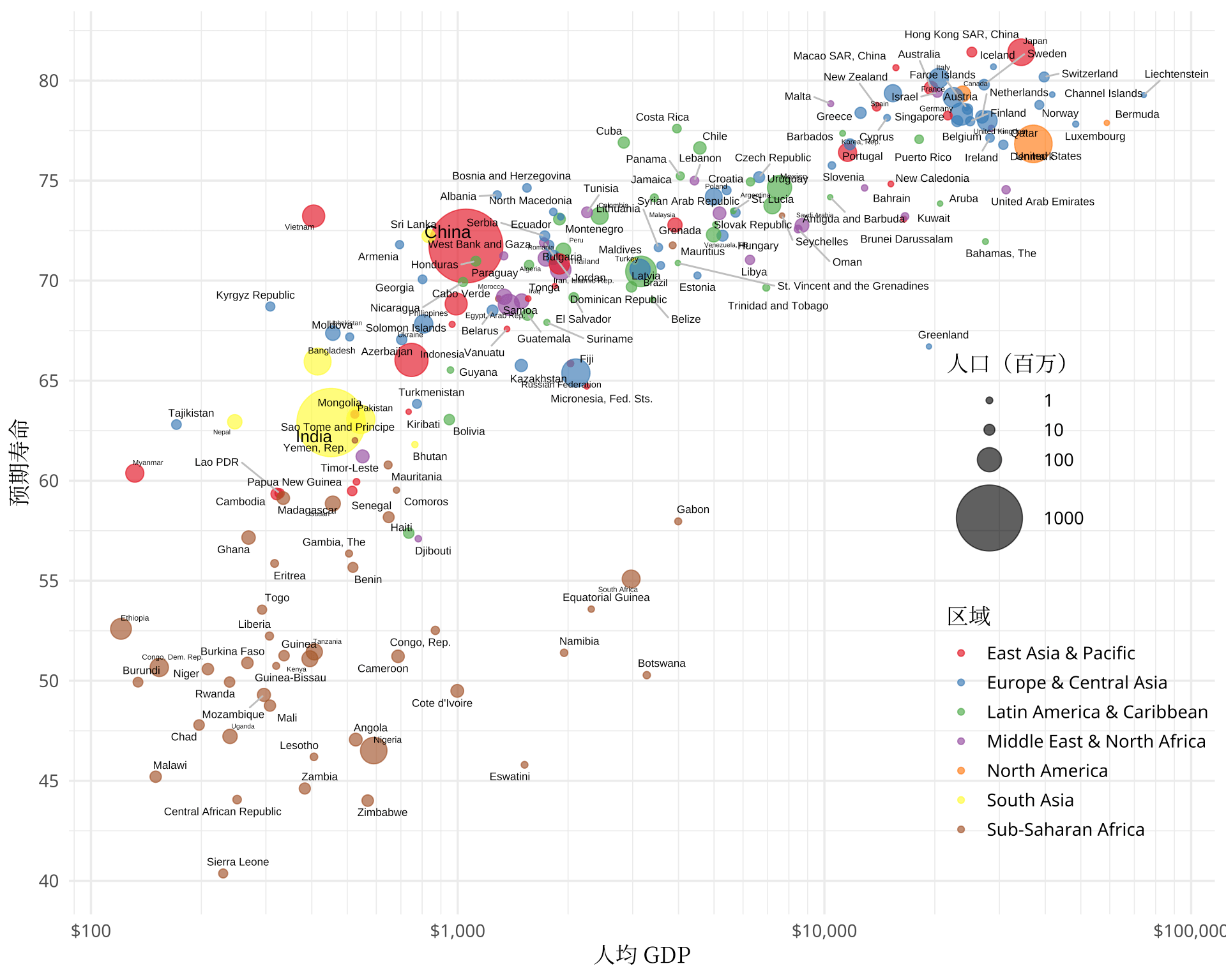
图 4: 2001 年寿命和人均 GDP 的关系
如图所示,撒哈拉以南的非洲地区人均 GDP 低、预期寿命短,南亚稍高一些,东亚及太平洋、欧洲及中亚地区人均 GDP 和预期寿命跨度大,比如日本、新加坡、香港、澳门等地区步入发达国家的水平,中东及北非地区人均 GDP 跨度也不小。北美都是发达国家,拉美集中在中等收入水平。世界银行还提供了国家收入水平的划分,如图5所示,以分面的形式可以更加清楚地展示各个地区的预期寿命和人均 GDP 的关系。
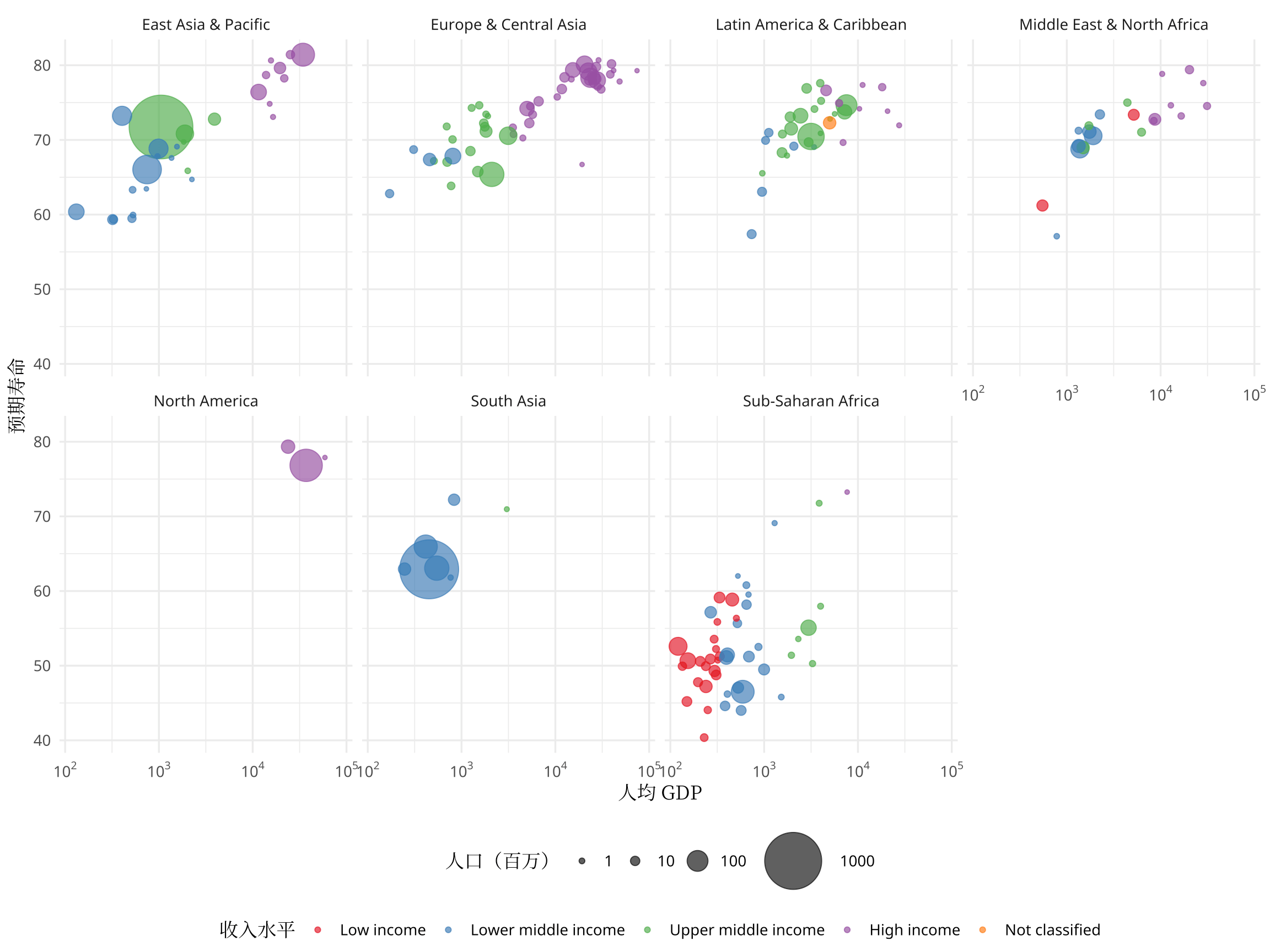
图 5: 2001 年寿命和人均 GDP 的关系(分地区)
点击显示或隐藏代码
wb_hans_2001$income_level <- factor(
  wb_hans_2001$income_level,
  labels = c("Low income", "Lower middle income", "Upper middle income", "High income", "Not classified"),
  levels = c("Low income", "Lower middle income", "Upper middle income", "High income", "Not classified")
)
ggplot(
  data = wb_hans_2001,
  aes(x = NY.GDP.PCAP.CD, y = SP.DYN.LE00.IN)
) +
  geom_point(aes(size = SP.POP.TOTL / 10^6, color = income_level), alpha = 0.7, na.rm = TRUE) +
  scale_x_log10(labels = scales::label_log()) +
  scale_color_brewer(palette = "Set1") +
  scale_size(breaks = c(1, 10, 100, 1000), range = c(1, 20)) +
  facet_wrap(~region, ncol = 4) +
  labs(
    x = "人均 GDP", y = "预期寿命",
    size = "人口(百万)", color = "收入水平"
  ) +
  theme_minimal(base_family = "Noto Sans", base_size = 13) +
  theme(
    title = element_text(family = "Noto Serif CJK SC"),
    legend.position = "bottom", legend.box = "vertical",
    legend.margin = margin()
  )
2001 年世界各地区人均 GDP 分布图
GDP 和人均 GDP 指标是官媒宣传最多的,各国希望营造一个橄榄球状的收入结构。在上一节可以粗略看出人均 GDP 将各个国家划分为收入不同的群体,下面采用密度估计图展示全世界收入的分布。如图6所示,横轴表示人均 GDP,纵轴表示国家数量,不同区域的人均 GDP 的分布,世界总的人均 GDP 的分布都展示出来了,国家层面,收入阶层的划分非常清晰。撒哈拉以南的国家或地区集中在人均 500 美元左右的区间里,少量达到 5000 美元的,极少量达到 10000 美元的。
点击显示或隐藏代码
mb <- unique(as.numeric(1:10 %o% 10^(1:4)))
ggplot(
  data = wb_hans_2001,
  aes(x = NY.GDP.PCAP.CD, y = stat(density * n), fill = region)
) +
  geom_density(position = "stack", colour = "white", na.rm = TRUE, alpha = 0.7) +
  scale_fill_brewer(palette = "Set1") +
  scale_x_log10(
    labels = scales::label_dollar(),
    limits = c(50, 300000),
    minor_breaks = mb) +
  labs(
    x = "人均 GDP", y = "国家数量", fill = "区域"
  ) +
  theme_minimal(base_family = "Noto Sans", base_size = 13) +
  theme(
    title = element_text(family = "Noto Serif CJK SC"),
    legend.position = "bottom"
  )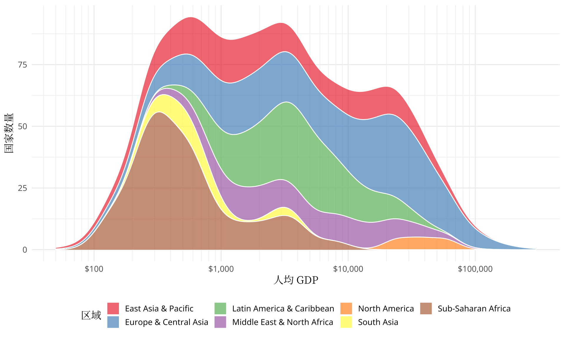
图 6: 2002 年世界人均 GDP 的分布
相信大家对「二八定律」不陌生,简单讲就是 20% 的人口占有全世界 80% 的财富,在经济社会等领域广泛存在。下面根据世界银行的数据,简单统计一下:
aggregate(wb_hans_2001, cbind(NY.GDP.PCAP.CD, SP.POP.TOTL) ~income_level, sum, na.rm = TRUE)
#          income_level NY.GDP.PCAP.CD SP.POP.TOTL
# 1          Low income          11388   3.378e+08
# 2 Lower middle income          48347   2.488e+09
# 3 Upper middle income         139982   2.199e+09
# 4         High income        1445793   1.059e+09
# 5      Not classified           4987   2.465e+07
贫穷的低收入国家和中低收入国家占有世界的财富比例为 3.619% 而人口占比为 46.27%。即近一半的人口占有的财富不足 4%。而高收入国家占有的财富比例为 87.6%,相应的人口占比为 17.34%,即不需要 20% 的人口就远远占据了 80% 的财富,比二八更狠!
数据展示
先准备各个年份的历史数据,从之前获取的大数据集中 wb_world_indicator 抽取一部分:
wb_hans <- subset(
  x = wb_world_indicator,
  subset = indicator_id %in% c("SP.DYN.LE00.IN", "NY.GDP.PCAP.CD", "SP.POP.TOTL"),
  select = c("date", "country", "region", "value", "indicator_id")
)
将「长格式」的数据重塑成「宽格式」的数据:
wb_hans <- reshape(
  data = wb_hans,
  varying = c("SP.POP.TOTL", "NY.GDP.PCAP.CD", "SP.DYN.LE00.IN"),
  timevar = "indicator_id",
  idvar = c("date", "country", "region"),
  direction = "wide"
)
wb_hans <- wb_hans[order(wb_hans$date), ]
查看变形重塑后的数据样子:
head(wb_hans)
#      date        country                     region SP.POP.TOTL NY.GDP.PCAP.CD
# 105  1960    Afghanistan                 South Asia     8996967          59.77
# 1260 1960        Albania      Europe & Central Asia     1608800             NA
# 1686 1960        Algeria Middle East & North Africa    11057864         246.30
# 2477 1960 American Samoa        East Asia & Pacific       20127             NA
# 3300 1960        Andorra      Europe & Central Asia       13410             NA
# 3695 1960         Angola         Sub-Saharan Africa     5454938             NA
#      SP.DYN.LE00.IN
# 105           32.45
# 1260          62.28
# 1686          46.14
# 2477             NA
# 3300             NA
# 3695          37.52
世界各地区人均 GDP 分布图
汉斯在 TED 演讲中还展示了另一幅世界各国人均 GDP 的分布动画,效果类似下图7。站在 ggplot2 和 gganimate 的肩膀上,有了前面的经验,制作起来不难,感兴趣的读者可查看代码复现。
点击显示或隐藏代码
library(gganimate)
mb <- unique(as.numeric(1:10 %o% 10^(1:4)))
ggplot(
  data = wb_hans,
  aes(x = NY.GDP.PCAP.CD, y = stat(density * n), fill = region)
) +
  geom_density(
    position = "stack", colour = "white",
    na.rm = TRUE, alpha = 0.7
  ) +
  scale_fill_brewer(palette = "Set1") +
  scale_x_log10(
    labels = scales::label_dollar(),
    limits = c(10, 350000),
    minor_breaks = mb
  ) +
  labs(
    title = "{frame_time} 年", fill = "区域",
    x = "人均 GDP", y = "国家数量"
  ) +
  theme_minimal(base_family = "Noto Sans", base_size = 13) +
  theme(
    title = element_text(family = "Noto Serif CJK SC"),
    legend.position = "bottom"
  ) +
  transition_time(date)
图 7: 世界各地区人均 GDP 分布图
有点佩服汉斯的想象力,他把多峰状态下的分布图看作是👻在摆手,中低收入国家形成的两座山峰正像👻一样步步逼近欧美等发达国家,最终,多峰几乎变成了单峰。
笔者此次从世界银行收集了 1960 年至今的历史数据,在图6 的基础上,下面拉长时间跨度,以岭线图观测过去 60 年世界收入的变化。二战以后,整体上,世界以和平与发展为主题,你好我好大家好,一起把人均 GDP 搞上去,对数化人均 GDP 数据后,其分布正朝着正态型曲线的方向迈进。特别地,2001 年全球化加速,高收入和中高收入国家之间的大峡谷正在逐渐消失,很多中低收入国家的人均 GDP 迈进了 10000 美元的大门,终于成了万元户,不过距离以美国为代表的发达国家仍然有 8-10 倍的差距。
点击显示或隐藏代码
library(ggridges)
mb <- unique(as.numeric(1:10 %o% 10^(1:4)))
ggplot(
  data = wb_hans, aes(x = NY.GDP.PCAP.CD, y = date, group = date)
) +
  geom_density_ridges(scale = 10, size = 0.25, rel_min_height = 0.03, na.rm = TRUE) +
  scale_x_log10(
    labels = scales::label_dollar(), n.breaks = 6,
    minor_breaks = mb
  ) +
  scale_y_reverse(n.breaks = 10) +
  labs(
    x = "人均 GDP", y = "年份"
  ) +
  theme_minimal(base_family = "Noto Sans", base_size = 13) +
  theme(
    title = element_text(family = "Noto Serif CJK SC"),
    axis.ticks = element_line(size = 0.5)
  )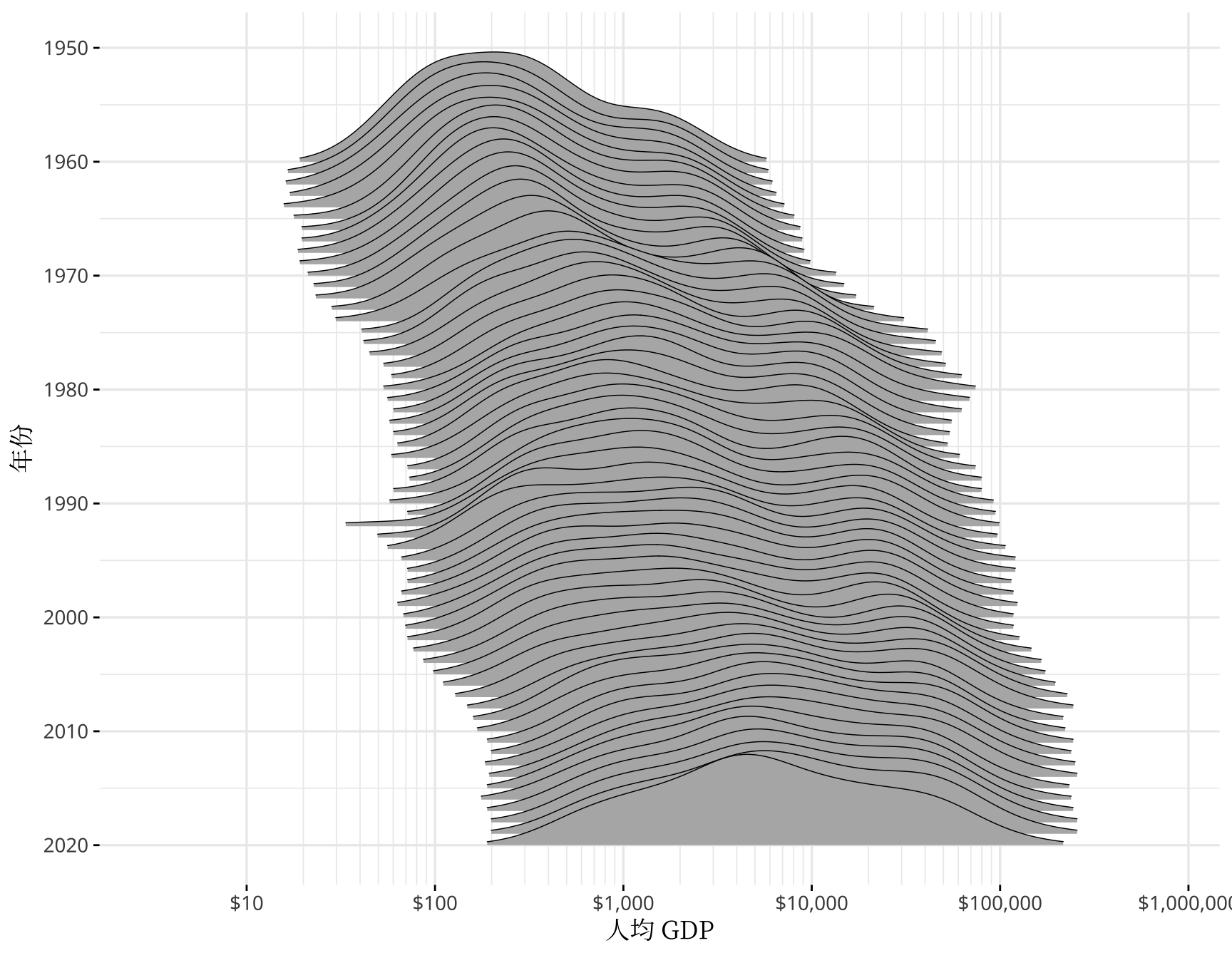
图 8: 世界人均 GDP 分布图
预期寿命与人均 GDP 的关系
GIF 动图的好处是便携,但没有暂停键,只有重复播放。下面用 echarts4r 包制作面向网页展示的动态气泡图,随时暂停和播放,还可回看,点击具体的气泡还可查看数据细节。交互式动态图的好处就是多,不过,制作起来也麻烦一些。一些常用的技术细节在另一篇文章《R 语言制作地区分布图及其动画》制作Web 动画部分介绍过了。下面捡几个重点介绍,其一添加动画标题和水印背景,这可以让读者更加醒目地看到当前状态,用 e_timeline_serie() 配置一些时间线组件的参数,参数是一个嵌套的列表结构,非常适合用 Base R 自带的函数 lapply() 来实现。
library(echarts4r)
# 去掉不完整的数据集
wb_hans <- wb_hans[complete.cases(wb_hans), ]
# 准备动画标题
titles <- lapply(unique(wb_hans$date), FUN = function(x) {
  list(
    text = paste(x, "年寿命与人均GDP关系", sep = ""),
    left = "center"
  )
})
# 准备动画背景文字
years <- lapply(unique(wb_hans$date), FUN = function(x) {
  list(
    subtext = x,
    left = "center",
    top = "center",
    z = 0,
    subtextStyle = list(
      fontSize = 100,
      color = "rgb(170, 170, 170, 0.5)",
      fontWeight = "bolder"
    )
  )
})
其二用颜色填充各个气泡,在 wb_hans 数据集上添加一列 color,根据国家所在的区域分配不同的颜色,颜色取自 RColorBrewer 包内置的 Spectral 调色板。各区域和颜色的对应关系可自定义,调整 levels 或 labels 里面的顺序即可,读者也可调用其它调色板。
wb_hans <- within(wb_hans, {
  color <- factor(
    region,
    levels = c(
      "East Asia & Pacific", "Europe & Central Asia",
      "Latin America & Caribbean", "Middle East & North Africa",
      "North America", "South Asia", "Sub-Saharan Africa"
    ),
    labels = RColorBrewer::brewer.pal(n = 7, name = "Spectral")
  )
})准备工作就绪后,绘制动画,效果如图9。
点击显示或隐藏代码
wb_hans |>
  group_by(date) |>
  # 横轴是人均 GDP
  e_charts(x = NY.GDP.PCAP.CD, timeline = TRUE) |>
  e_scatter(
    # 纵轴是人均寿命(预期寿命)
    serie = SP.DYN.LE00.IN,
    # 气泡大小表示人口总数
    size = SP.POP.TOTL,
    # 国家名称
    bind = country,
    # 气泡的样式
    symbol = "circle",
    # 气泡大小的 base 参照值
    symbol_size = 5,
    # 设置气泡的透明度,缓解重叠现象
    itemStyle = list(opacity = 0.8),
    # 去掉图例标题,为主标题腾位置
    name = ""
  ) |>
  # 填充气泡颜色
  e_add_nested("itemStyle", color) |>
  e_y_axis(
    min = 20, max = 90,
    # 纵轴标题到轴线的距离
    nameGap = 40,
    # 纵轴标题
    name = "人均寿命",
    # 纵轴标题位置
    nameLocation = "center",
    # 纵轴标题样式
    nameTextStyle = list(fontWeight = "bold", fontSize = 18)
  ) |>
  e_x_axis(
    # 设置横轴为对数尺度,默认以10为底
    type = "log",
    min = 10, max = 100000,
    # 以 10 为底的对数
    logBase = 10,
    minorSplitLine = list(show = TRUE),
    minorTick = list(show = TRUE, splitNumber = 10),
    nameGap = 30, name = "人均 GDP",
    nameLocation = "center",
    nameTextStyle = list(fontWeight = "bold", fontSize = 18)
  ) |>
  e_tooltip(
    # 定制悬浮内容
    # params.name 取自 bind 变量
    formatter = htmlwidgets::JS("
      function(params) {
        if(params.value) {
          return('国家: <strong>' + params.name + '</strong>' +
                 '<br />人均 GDP: ' + Math.round(params.value[0]) + '美元' +
                 '<br />人均寿命: ' + Math.round(params.value[1]) + '岁' +
                 '<br />人口总数: ' + Math.round(params.value[2] / 1000000 * 100) / 100 + '百万')
        } else {
          return('');
        }
      }
    ")
  ) |>
  # 刻度单位
  e_format_x_axis(suffix = "美元") |>
  e_format_y_axis(suffix = "岁") |>
  # 动画的主标题
  e_timeline_serie(title = titles, index = 1) |>
  # 动画的背景年份
  e_timeline_serie(title = years, index = 2) |>
  # 动画设置
  e_timeline_opts(
    autoPlay = FALSE, # 自动播放动画
    playInterval = 500, # 播放的速度,单位毫秒
    loop = TRUE, # 是否循环播放动画
    show = TRUE
  ) |>
  # 坐标系内网格距离容器下方的距离
  e_grid(bottom = 100)
图 9: 致敬 Gapminder
最后,补充几个细节点:
快速制作一个带时间轴的气泡图10是不难的,这就相当于图形主体内容都有了。
点击显示或隐藏代码
wb_hans |>
  group_by(date) |>
  # 横轴是人均 GDP
  e_charts(x = NY.GDP.PCAP.CD, timeline = TRUE) |>
  e_scatter(
    # 纵轴是人均寿命(预期寿命)
    serie = SP.DYN.LE00.IN,
    # 气泡大小表示人口总数
    size = SP.POP.TOTL,
    # 国家名称
    bind = country,
    # 气泡的样式
    symbol = "circle",
    # 气泡大小的 base 参照值
    symbol_size = 5,
    # 设置气泡的透明度,缓解重叠现象
    itemStyle = list(opacity = 0.8),
    # 用于tooltip的显示,legend 的图例筛选
    name = "Gapminder"
  ) |>
  e_x_axis(
    # 设置横轴为对数尺度,默认以10为底
    type = "log",
    min = 10, max = 100000
  ) |>
  e_y_axis(
    min = 20, max = 90
  ) |>
  e_tooltip()
图 10: 预期寿命与人均 GDP 的关系变化
echarts4r 包提供的
group_by()函数只支持传入一个变量,用作动画的时间帧变量。如下方式传入多个变量也无法实现分组效果,上面的动画9是通过添加函数e_add_nested()修改 itemStyle 实现的。这得感谢苏玮在论坛解答我关于 echarts4r 包的使用问题。wb_hans |> group_by(date, region)对照 Apache ECharts 时间线 组件的帮助文档,echarts4r 有的参数名称和 Apache ECharts 略微不同,函数
e_timeline_opts()的axis_type对应axisType,e_timeline_serie()的index对应currentIndex。次刻度线设置的参照坐标轴文档,
splitNumber参数控制次刻度线分割数。图中设为 10,次刻度线由疏到密,这是对数函数决定的。log(seq(from = 100, to = 1000, by = 100), base = 10) # [1] 2.000 2.301 2.477 2.602 2.699 2.778 2.845 2.903 2.954 3.000动画里,大气泡覆盖小气泡,尽管设置了透明度,可以看到小气泡的位置,但是鼠标悬浮在小气泡上时,无法显示小气泡上的悬浮文本,这很有可能是 Apache ECharts 的问题,因为官方示例也有此问题。一种可能的缓解办法是把数据集按人口总数切分成两块,先画大气泡,再画小气泡,笔者没有尝试。
鼠标落在时间轴上,悬浮提示包含整个自定义
e_tooltip()内容,这是有问题的,笔者还没找到解决办法。
点击显示或隐藏代码
wb_hans <- within(wb_hans, {
  life <- round(SP.DYN.LE00.IN, 2)
})

wb_hans |>
  group_by(date) |>
  e_charts(country, timeline = TRUE) |>
  e_map(serie = life, name = "预期寿命") |>
  e_visual_map(
    min = 15, max = 90,
    inRange = list(
      color = RColorBrewer::brewer.pal(n = 11, name = "RdBu")
    )
  ) |>
  e_tooltip() |>
  e_timeline_opts(
    autoPlay = FALSE, # 自动播放
    show = TRUE, # 展示时间轴
    playInterval = 1000 # 转场时间
  )
图 11: 预期寿命
点击显示或隐藏代码
wb_hans <- within(wb_hans, {
  log_gdp <- round(log(NY.GDP.PCAP.CD, base = 10), 2)
})

wb_hans |>
  group_by(date) |>
  e_charts(country, timeline = TRUE) |>
  e_map(serie = log_gdp, name = "人均 GDP(对数)") |>
  e_visual_map(
    min = 1, max = 6,
    inRange = list(
      color = RColorBrewer::brewer.pal(n = 11, name = "RdBu")
    )
  ) |>
  e_tooltip() |>
  e_timeline_opts(
    autoPlay = FALSE, # 自动播放
    show = TRUE, # 展示时间轴
    playInterval = 1000 # 转场时间
  )
图 12: 人均 GDP(单位:美元,取10为底的对数)
点击显示或隐藏代码
wb_hans2 <- within(wb_hans, {
  log_gdp <- round(log(NY.GDP.PCAP.CD, base = 10), 2)
  country <- ifelse(country == "Russian Federation", "Russia", country)
  country <- ifelse(country == "Congo, Dem. Rep.", "Dem. Rep. Congo", country)
  country <- ifelse(country == "Central African Republic", "Central African Rep.", country)
  country <- ifelse(country == "Congo, Rep.", "Congo", country)
  country <- ifelse(country == "South Sudan", "S. Sudan", country)
  country <- ifelse(country == "Egypt, Arab Rep.", "Egypt", country)
  country <- ifelse(country == "Iran, Islamic Rep.", "Iran", country)
  country <- ifelse(country == "Yemen, Rep.", "Yemen", country)
})

wb_hans2 |>
  group_by(date) |>
  e_charts(country, timeline = TRUE) |>
  e_map(serie = log_gdp, name = "人均 GDP(对数)") |>
  e_visual_map(
    min = 1, max = 6,
    inRange = list(
      color = RColorBrewer::brewer.pal(n = 11, name = "RdBu")
    )
  ) |>
  e_tooltip() |>
  e_timeline_opts(
    autoPlay = FALSE, # 自动播放
    show = TRUE, # 展示时间轴
    playInterval = 1000 # 转场时间
  )
图 13: 人均 GDP(单位:美元,取10为底的对数)
本文小结
世界上没有两片相同的叶子,差异是始终存在的,统计上的显著性差异是需要从万千变化中筛选出来的。相比于理解变化,关注差异是容易的。
在数据分析方面,还有很多有意思的话题值得探索分析:
- 从数据上看,中国是否有进入「中等收入陷阱」的迹象?
- 有人说,中国在2035年以后将迎来的不是人口老龄化「高峰」而是人口老龄化「高原」,这是否有数据依据?
- 是不是人均 GDP 上去了,人口增长率就会下降?人口问题由经济因素主导还是意识形态主导?
- 有人说 GDP 的高速增长会掩盖很多社会经济问题,只有潮水退去才知道是谁在裸泳,GDP 增长越快是不是失业率越低?
- 越是宏观的越是复杂,事关居民生活的通货膨胀率、消费价格指数到底受什么波动?
大势是由国家、行业决定的,选择一个行业方向是个人可以做的,很多人说选择比努力重要,站在风口上猪都能飞起来,人这一生能做一次风口上的猪就足够了。这么看,这套选择的方法论非常类似商业分析框架,基本面(宏观)、行业(中观)、企业(微观)都要看。那么多的行业、那么多的变量,这个变量选择一定是超高维的,仅凭一人之力,还是着眼当下,了解自己。
在技术实现方面,稍微扩展一下,动态图形包含动图、动画、影视等一切可以自动播放一帧帧画面的图形图像,这就包含各种各样的形式,如 GIF 动图,SWF 动画,MP4 视频,以及网页渲染的动画,当然还有三维动画。除了本文介绍的两个制作动画的 R 包,R 社区还有一些 R 包有制作动画的能力,如表1所示。笔者精力和时间有限,感兴趣的读者不妨试试其它的技术实现。
| R 包 | 简介 |
|---|---|
| animation | A Gallery of Animations in Statistics and Utilities to Create Animations |
| echarts4r | Create Interactive Graphs with ‘Echarts JavaScript’ Version 5 |
| gganimate | A Grammar of Animated Graphics |
| magick | Advanced Graphics and Image-Processing in R |
| plotly | Create Interactive Web Graphics via ‘plotly.js’ |
| rayrender | Build and Raytrace 3D Scenes |
| rgl | 3D Visualization Using OpenGL |
Python 的 plotly 模块功能比 echarts4r 的还多,在统计和易用性方面也强很多,更多详情见文章《动画制作与 Plotly Python》。
图 14: 基于 gapminder 数据用 plotly 复现汉斯·罗琳的动态气泡图
环境信息
在 RStudio IDE 内编辑本文的 R Markdown 源文件,用 blogdown (Xie, Hill, and Thomas 2017) 构建网站,Hugo 渲染 knitr 之后的 Markdown 文件,得益于 blogdown 对 R Markdown 格式的支持,图、表和参考文献的交叉引用非常方便,省了不少文字编辑功夫。文中使用了多个 R 包,为方便复现本文内容,下面列出详细的环境信息:
xfun::session_info(packages = c(
  "knitr", "rmarkdown", "blogdown",
  "echarts4r", "gganimate", "ggplot2",
  "ggridges", "ragg", "showtext",
  "wbstats", "gapminder", "ggrepel"
), dependencies = FALSE)
# R version 4.2.0 (2022-04-22)
# Platform: x86_64-apple-darwin17.0 (64-bit)
# Running under: macOS Big Sur/Monterey 10.16
#
# Locale: en_US.UTF-8 / en_US.UTF-8 / en_US.UTF-8 / C / en_US.UTF-8 / en_US.UTF-8
#
# Package version:
#   blogdown_1.10   echarts4r_0.4.4 gapminder_0.3.0 gganimate_1.0.7
#   ggplot2_3.3.6   ggrepel_0.9.1   ggridges_0.5.3  knitr_1.39
#   ragg_1.2.2      rmarkdown_2.14  showtext_0.9-5  wbstats_1.0.4
#
# Pandoc version: 2.18
#
# Hugo version: 0.98.0